

not logged in | [Login]
![]()
This module generates both a heat demand density and a gross floor area density map in the form of raster files. The input to the module are different development scenarios of the heat demand and gross floor areas at national levels and broken down to each raster element as well as user-defined parameters to describe the relative deviation to the developments in the scenarios.
For the analysis of the future potentials for the supply of heat and cold from renewable and excess heat sources, it is essential to take into account potential developments in the building stock of the analysed region. Part of the buildings are renovated in order to decrease energy demand for space heating, part of the buildings are demolished and new buildings are constructed. This leads to changes in the heat demand of the buildings in a region. Furthermore, the evolution of the population and the Gross Domestic Product (GDP) in a region influences the development of the demand for building gross floor area and thus the demand for space heating and hot water generation. The aim of the Calculation Module (CM) - Demand Projection is to provide scenarios of the future development of gross floor areas and heat demand in buildings for a selected area based on calculations for the EU-28 at the national level. Different scenarios, which are calculated using the Invert/EE-Lab module, are broken down on the level of hectares. They differ in their thermal renovation rate, in other words how much of the gross floor area is renovated proportionally. The CM also provides the opportunity to change three basic drivers in the scenarios and generate adapted results. These three basic drivers are a) the reduction of the gross floor area of existing buildings, b) the reduction of the specific energy needs in the buildings, and c) the annual population growth addition to default growth
Select scenario:
Select target year:
Reduction of gross floor area compared to the reference scenario:
Reduction of specific energy needs compared to reference scenario:
Annual population growth in addition to default growth:
Method to add newly constructed buildings to the map:
Indicators:
Graphics:
Layers:
As written before this module is based on calculations performed with the Invert/EE-Lab module for all countries of the EU 28 (see www.invert.at for a description of the method of the Invert/EE-Lab module). The calculated scenarios are analysed regarding the development of the following types of buildings: residential and non-residential buildings, 3 construction periods and newly constructed buildings. Then the population growth per NUTS3 region and the initial building stock (in terms of heated gross floor area & energy needs per construction period and building type) per NUTS 3 region are assessed. Based on this assessment the results of the calculated scenarios are transferred to the respective NUTS3 region. The NUTS3 results are then distributed to the different hectare elements according to the method developed in Müller et al 2019 (REFERENCE).
The module provides 4 different scenarios, which vary in their renovation rates. Through a selection, either 0.5%, 1%, 2% or 3% of the total gross floor area is renovated annually. It is to be noted that the saved heating requirement is not directly proportional to an increase in the renovation rate since different effective renovations are permitted. With a small renovation rate, mainly buildings are renovated, where favourable measures can achieve large savings. With a high renovation rate, buildings with a higher thermal quality are also increasingly being renovated and their saved heating energy is lower in comparison. The base scenario behind the different scenarios is the reference scenario which is described in the following part.
"reference": Current efficiency policies remain in place and are effectively implemented. We assume that in general, building owners and professionals comply with regulatory instruments like building codes. National differences in the policy intensity continue to exist. Therefore, the policy intensity indicates qualitatively the range of policy ambition in different countries. The energy efficiency policy mix corresponds to the current packages in place, which in most countries is a mix of regulatory approaches (building codes, nearly zero energy buildings (nZEB) definitions, RES-H obligation), economic support (subsidies for building refurbishment) and energy taxation. Main sources for implemented policies are the Mure database (www.measures-odyssee-mure.eu/) and the projects ENTRANZE (www.entranze.eu/) and Zebra2020 (www.zebra2020.eu/). While the scenario considers neither a strong technology improvement nor binding energy efficiency obligations, ambitious policies to foster renewable energy are in place. This has been implemented based on mandatory renewable energy quotas on the level of individual buildings.
Energy prices: Energy prices increase moderately according to EU Reference Scenario 2016 (https://ec.europa.eu/energy/en/data-analysis/energy-modelling).
Technology development: The assumed technological learning is very low and costs for efficient and renewable heating/cooling technologies decrease only slightly.
Qualitative overview of policy assumptions:
Results: Total final energy demand for space heating, hot water, cooling, and auxiliary energy demand in EU-28 amounts to approximately 3850 TWh for all renovation rates in 2015 and decreases to 2800TWh to 2250 TWh in 2050, depending on the renovation rate.
EU-28:
 Figure: Final energy demand in EU-28 from 2015 to 2050 for different renovation rates
The following six graphs depict the development of the final energy demand for space heating, cooling, and domestic hot water preparation for the individual EU member states.
DE, FR, GB, IT and PL:
 Figure: Final energy demand in DE, FR, GB, IT and PL for 2015 and 2050 with different renovation rates
 Figure: Portion of Final energy demand in 2050 for DE, FR, GB, IT and PL relative to 2015
NL, ES, BE, SE, CZ, HU, AT, RO, FI, DK and GK:
 Figure: Final energy demand in NL, ES, BE, SE, CZ, HU, AT, RO, FI, DK and GK for 2015 and 2050 with different renovation rates
 Figure: Portion of Final energy demand in 2050 for NL, ES, BE, SE, CZ, HU, AT, RO, FI, DK and GK relative to 2015
SK, IE, PT, HR, BG, LT, LV, SI, EE, LU, CY and MT:
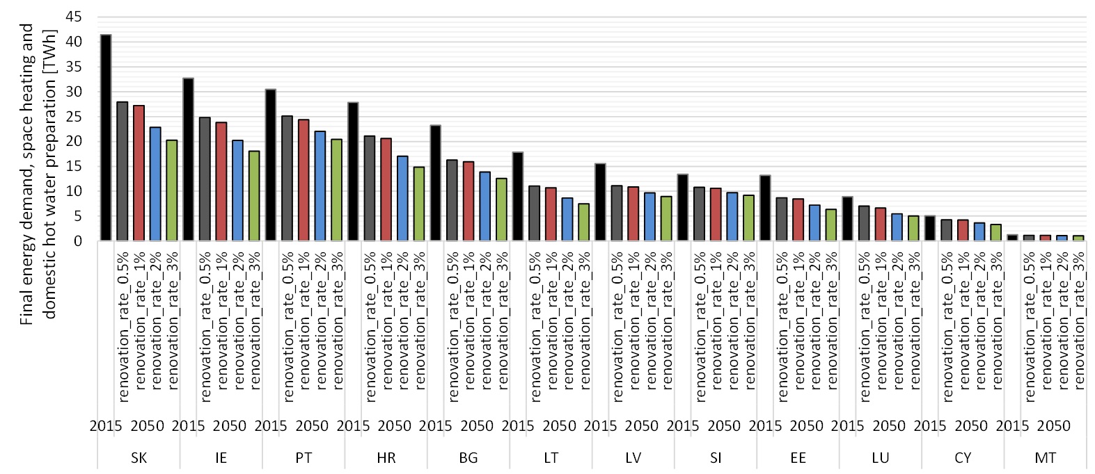 Figure: Final energy demand in SK, IE, PT, HR, BG, LT, LV, SI, EE, LU, CY and MT for 2015 and 2050 with different renovation rates
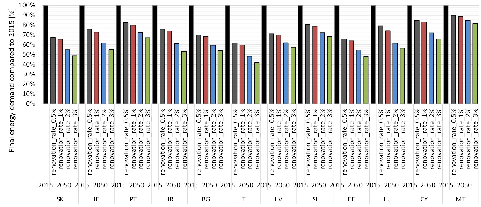 Figure: Portion of Final energy demand in 2050 for SK, IE, PT, HR, BG, LT, LV, SI, EE, LU, CY and MT relative to 2015
Here you get the bleeding-edge development for this calculation module.
Here, the calculation module is run for the case study of Vienna, Austria. First, use the "Go To Place" bar to navigate to Vienna and select the city. Click on the "Layers" button to open the "Layers" window and then click on the "CALCULATION MODULE" tab. In the list of calculation modules, select "CM - Demand projection".
The default input values generate a heat demand density map for 2017. These values should be regarded as starting point only. You may need to set values below or above default values considering additional local considerations. The scenario used also has a strong effect on the output. Therefore, the user should adapt these values to find the best combination of inputs for her or his case study.
To run the calculation module, follow the next steps:
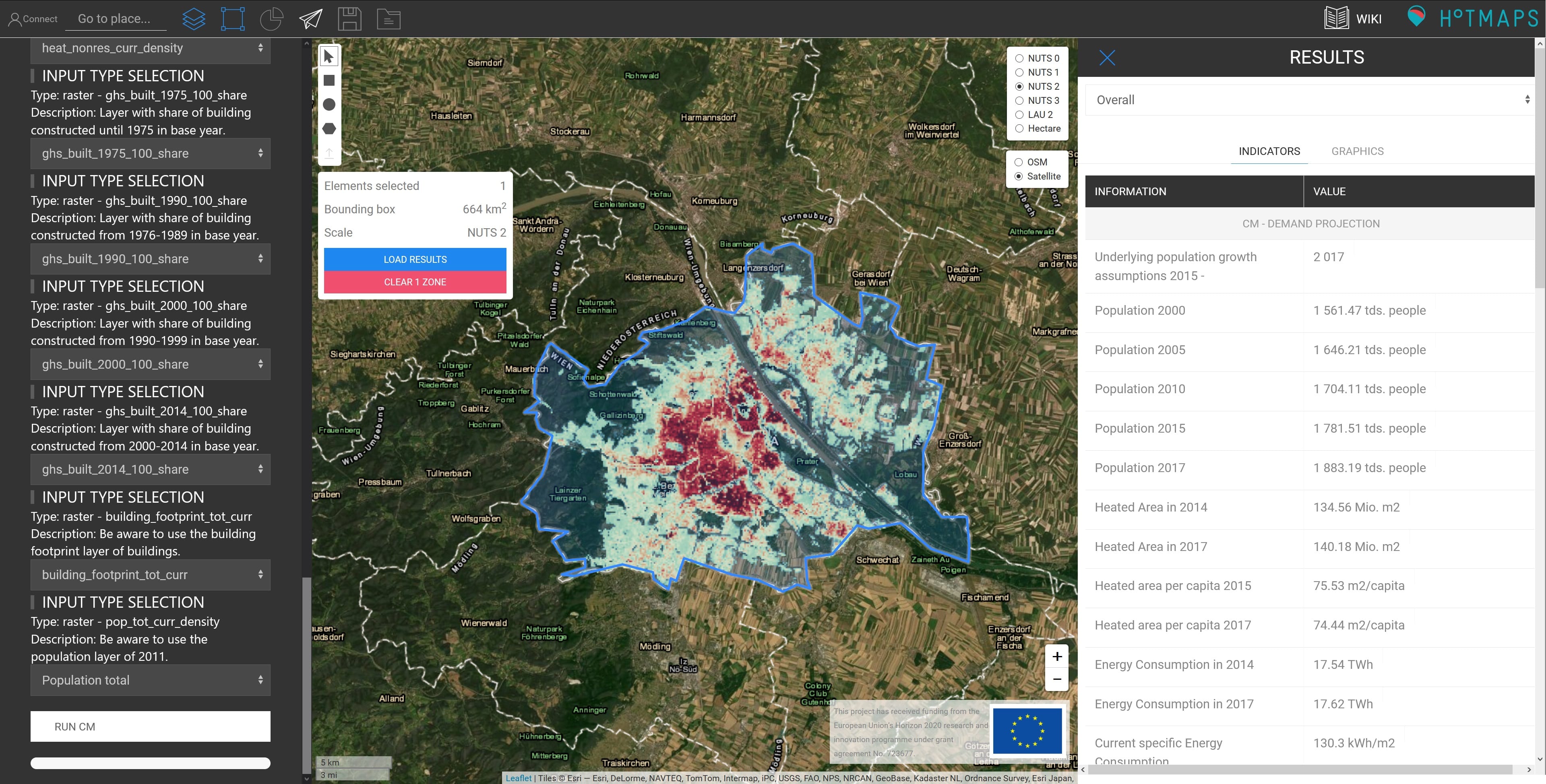 Figure: Demand projection after running with default parameter
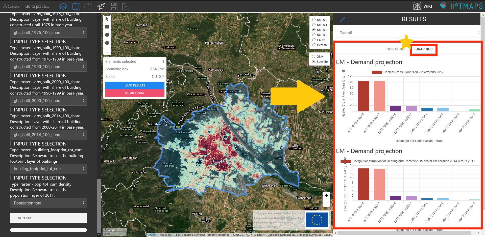 Figure: Demand projection after running with default parameter, switching to graphics
 Figure: Demand projection after running with default parameter, switching to result layers
As mentioned before, it may be necessary to adjust the input parameters to the own data situation or to check sensitivities.
Andreas Müller and Marcus Hummel, in Hotmaps-Wiki, CM-Demand-projection (October 2019)
This page was written by Andreas Müller and Marcus Hummel (e-think).
☑ This page was reviewed by Mostafa Fallahnejad (EEG - TU Wien).
Copyright © 2016-2020: Andreas Müller and Marcus Hummel
Creative Commons Attribution 4.0 International License
This work is licensed under a Creative Commons CC BY 4.0 International License.
SPDX-License-Identifier: CC-BY-4.0
License-Text: https://spdx.org/licenses/CC-BY-4.0.html
We would like to convey our deepest appreciation to the Horizon 2020 Hotmaps Project (Grant Agreement number 723677), which provided the funding to carry out the present investigation.
View in another language:
* machine translated